How to Create a Pivot Table in Excel in under 2 minutes!

Pivot tables are useful for summarizing and analyzing data in a compact, organized format. Scientists often have to work with large datasets, and pivot tables can help make sense of this data by aggregating and transforming it into meaningful information.

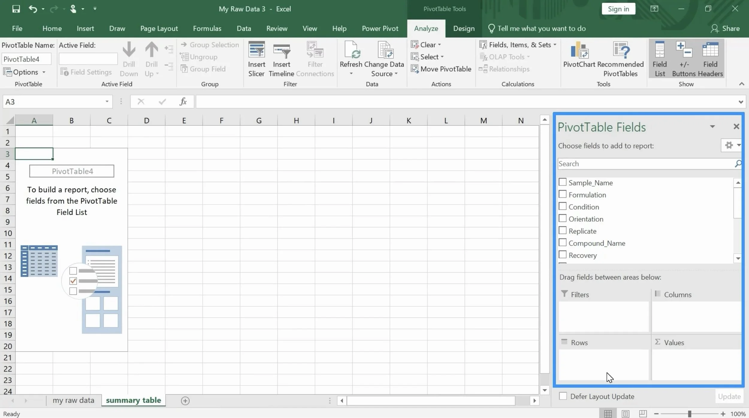
Step 1. Go to insert and click PivotTable. Excel will automatically select your entire data set. Choose New Worksheet to create the table in a new sheet. Click okay.

Step 2. On the right side of the sheet, we can see the pivot table fields pane. This is where we can configure the fields that we will use to build our table. We could drag and drop the following fields:

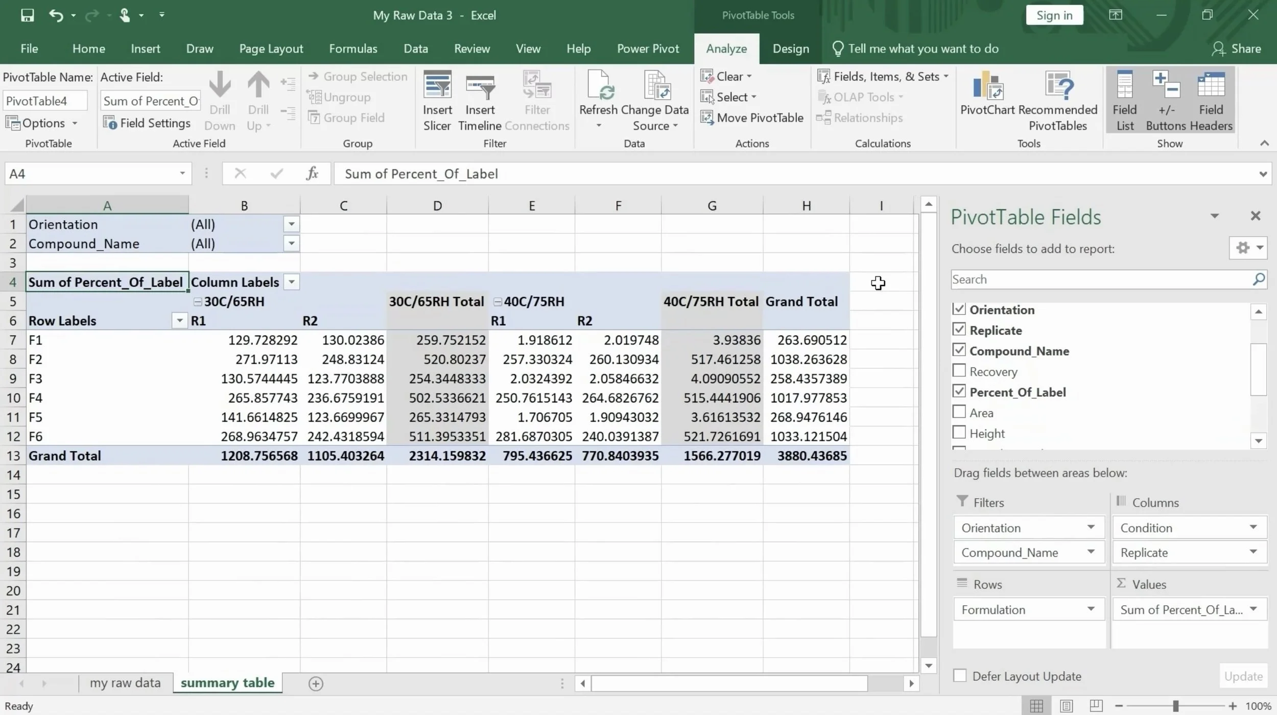
Formulations will be our rows

Condition and replicates will be our column headers

Orientation and compound name will be our filters

% of label will be our values

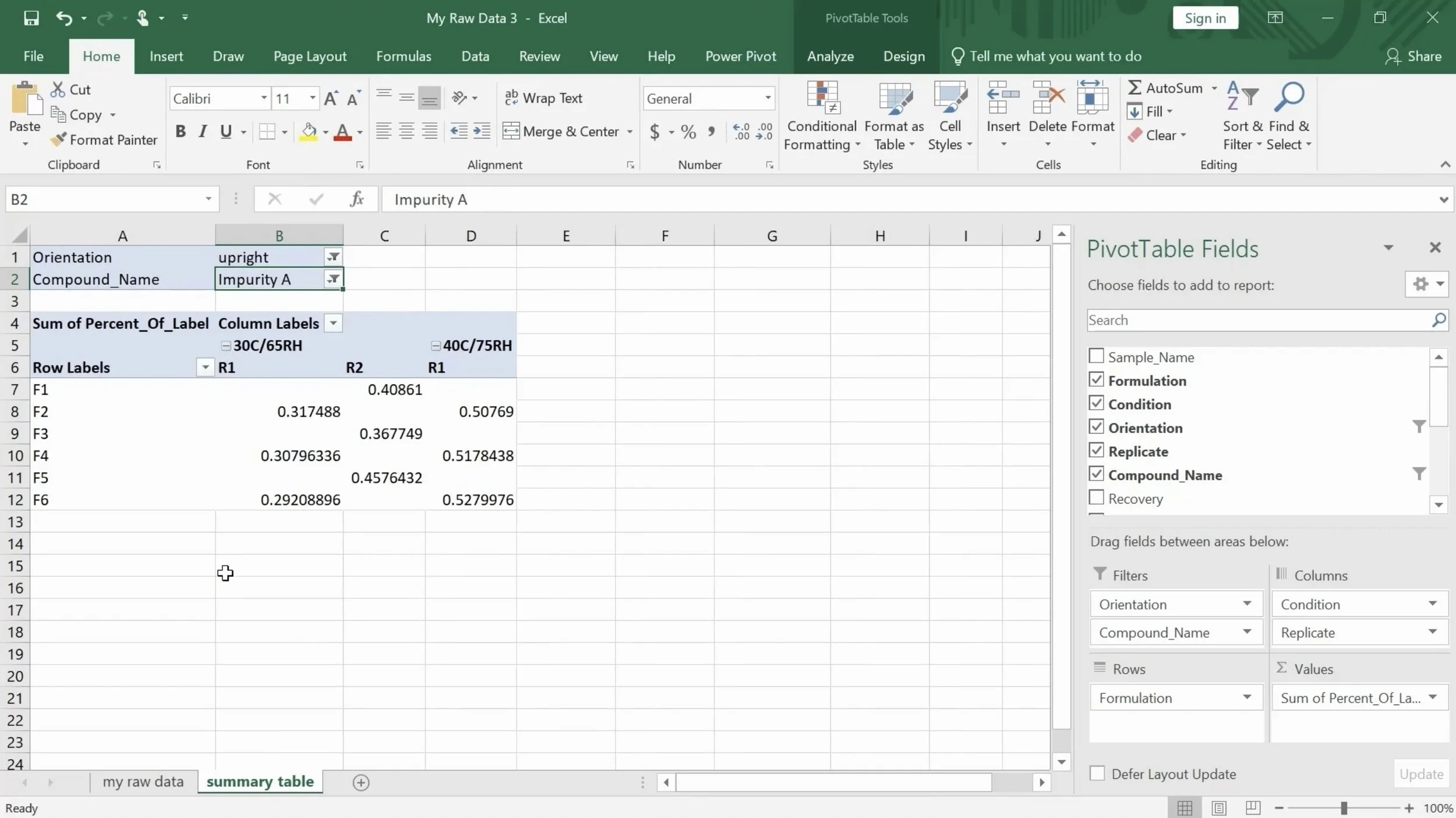
Here is the resulting table after dragging and dropping the fields:

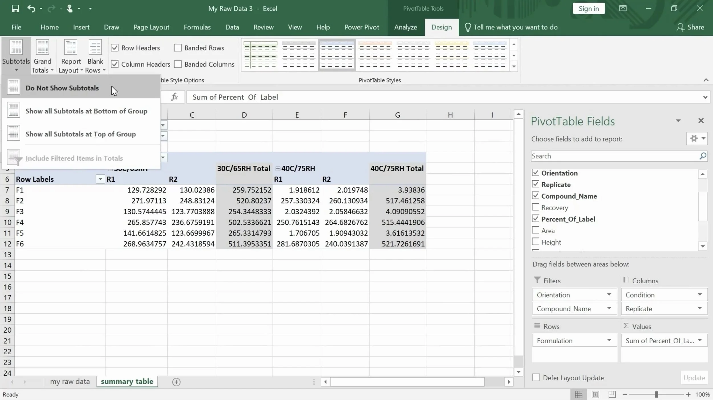
Step 3. To clean up our table, we can go to the pivot table design tab and remove the grand totals and subtotals

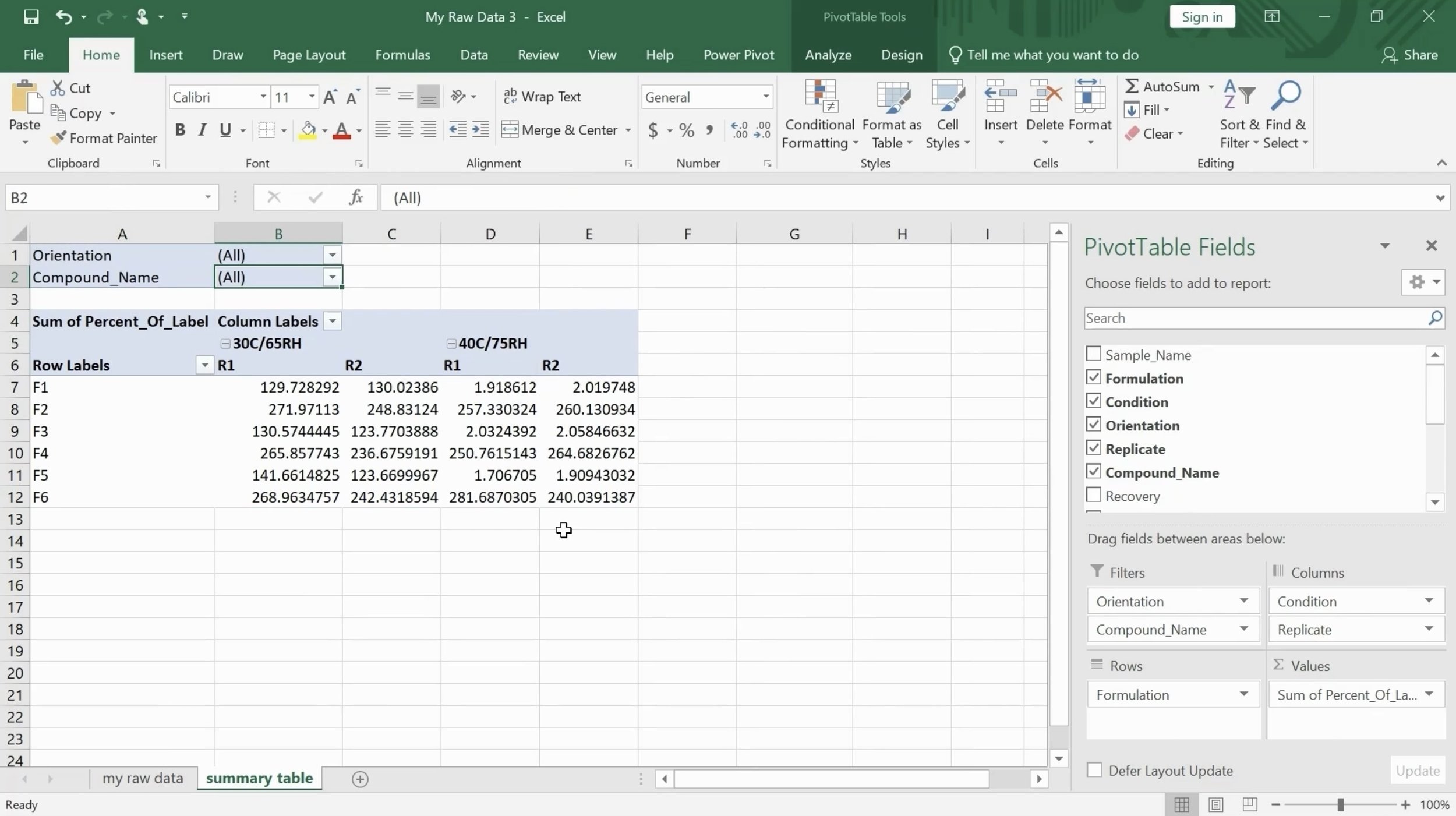
Step 4. Now we can change our orientation and compound name filters depending on what we want to display in our table. For orientation let’s choose upright and for compound let’s choose impurity A. And that’s it!

Do you have any questions or suggestions? Feel free to reach us by clicking here.