Locking your Columns and Rows Using Freeze Panes
When you have a large dataset and you scroll down through your data, you lose sight of the column headers at the top. Similarly, if you scroll to the right, you lose sight of the row labels on the left.
To keep your columns and rows in place, use freeze panes in just two easy steps!
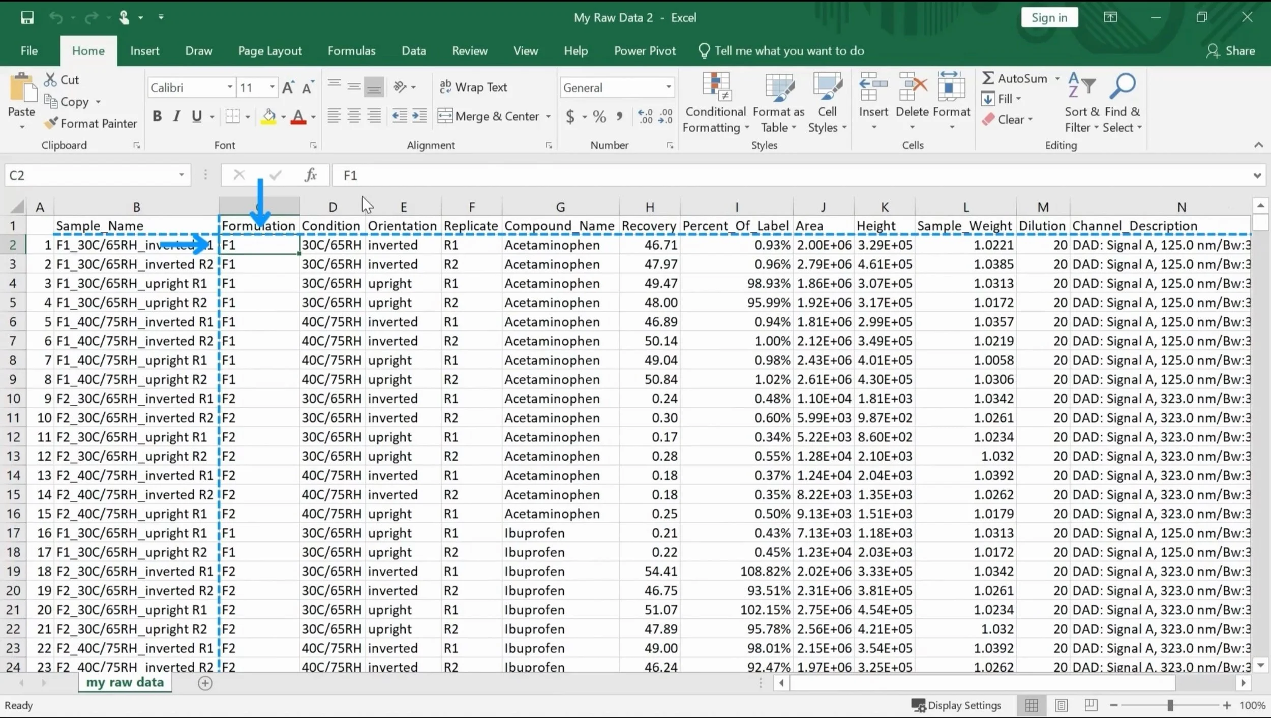
Step 1: Select the cell that is below the row and to the right of the column you want to freeze.
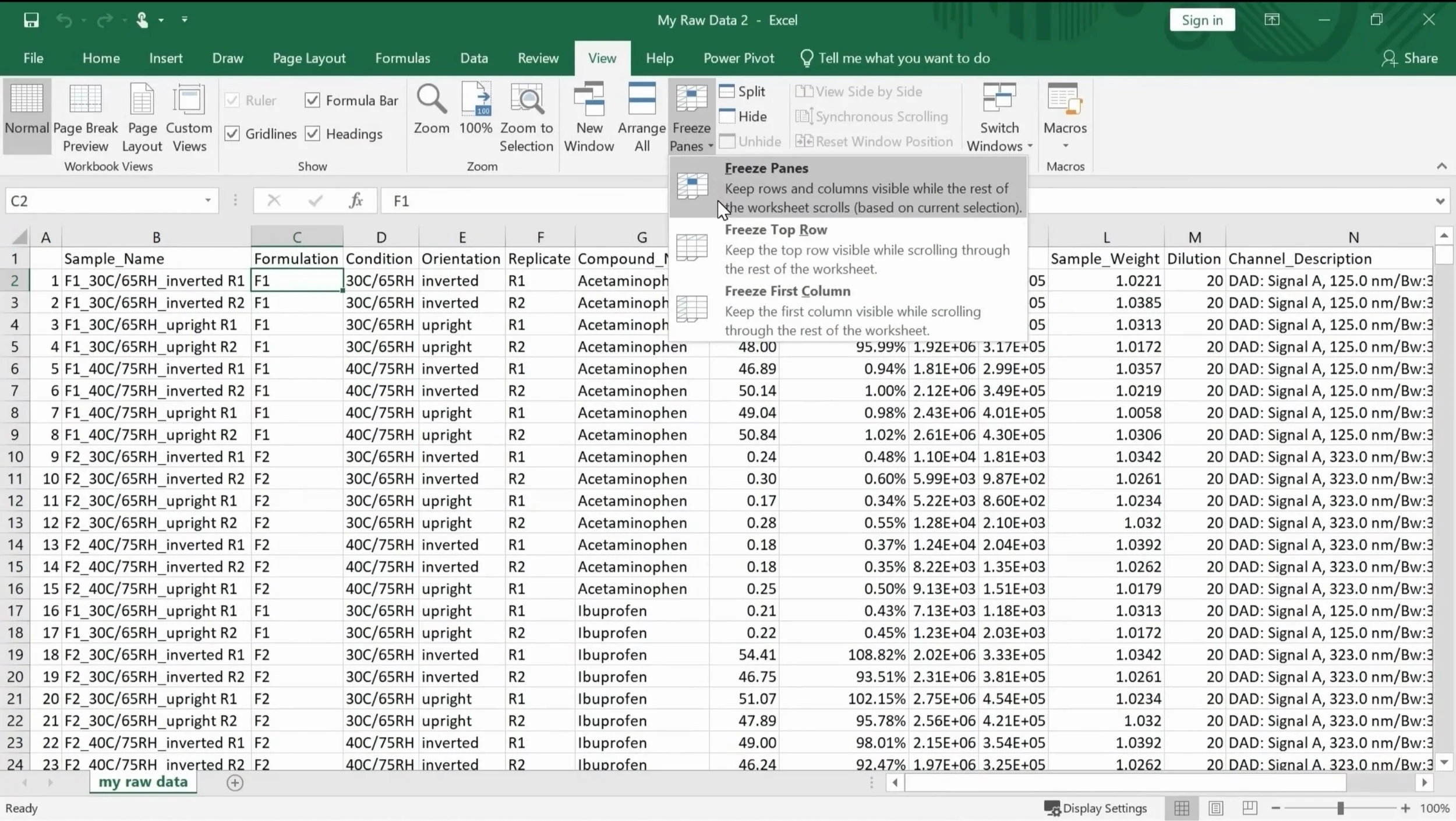
Step 2: Go to View. Click the Freeze Panes dropdown. Click on Freeze Panes.
And that’s it! The sample name column and the column headers are now locked!
Do you have any questions or suggestions? Feel free to reach us by clicking here.


